Getting started with PECCARY

The following example will walk you through the basic functions of the peccary package. Additional descriptions and examples for all functions and class can be found in the User Guide.

Initializing double pendulum system

First, import peccary (the core analysis of the package), examples (which can generate a variety of different timeseries), and HCplots (used for plotting on the \(HC\)-plane), as well as some additional packages:

>>> import numpy as np
>>> import matplotlib.pyplot as plt
>>> from peccary import peccary
>>> import peccary.examples as ex
>>> from peccary import HCplots
>>> from peccary import utils

Integration and initializing PECCARY

To start with PECCARY, you need some sort of timeseries to analyze. Let’s set up a double pendulum system where each mass is 1 kg and both rods are 1 meter long. To initialize it, we use:

>>> pendSys =  ex.doublePendulum(L1=1.0, L2=1.0, M1=1.0, M2=1.0)

Now let’s integrate the system for 10 seconds at a time resolution of \(2^{-6}:\) seconds (approx 0.016 seconds). Right now, we’ll just use the default initial angle and angular velocity conditions of \(\theta_1 = 120^{\circ}\), \(\theta_2 = -10^{\circ}\), and \(\omega_1 = \omega_2 = 0^{\circ} \textrm{s}^{-1}\), but these values can be changed with the th1, w1, th2, and w2 arguments of the function. We can do this with:

>>> pend = pendSys.integrate(tDur=10., dt=np.power(2.,-6.))

The resulting object of the integration is a Timeseries object, which wraps the timesteps, time resolution, and x- and y-coordinates into one object. You can call the time resolution with the attribute and print it out, e.g.,:

>>> print(pend.dt)
0.015625

We can check that everything looks right by plotting using the plotStatic method of the doublePendulum class. To do this, we apply this method to the pendSys class we initialized, and then input the Timeseries class returned by the integrate method, i.e.,:

>>> fig, ax = pendSys.plotStatic(pend)
>>> plt.show()

This gives us the plot:

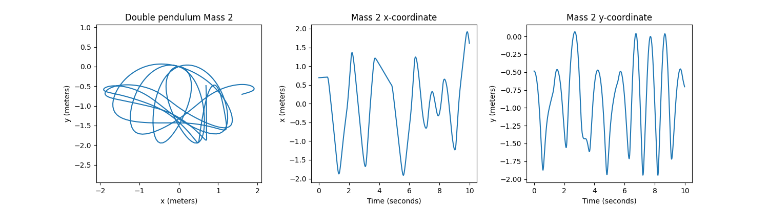
That looks good! Now, let’s run PECCARY on the x-coordinates of the second mass (mass 2) of our double pendulum system. Since the doublePendulum class stores x- and y-data for both masses in a Timeseries class, we need to specify that we want to analyze the x-coordinates for the the second particle (or mass) in the system:

>>> pecc = peccary(pend, attr='x', ptcl=1)

Calculating and plotting \(H\) and \(C\)

To run PECCARY for a range of sampling intervals, we use the calcHCcurves method. By default, it will run the analysis for sampling intervals from \(\ell = 1\) to \(\ell = 100\) at increments of 1. This can be changed via the min_sampInt, max_sampInt, and step_sampInt parameters or with the sampIntArray parameter.

Right now, we’ll just use the default parameters, to get:

>>> H, C, ells = pecc.calcHCcurves()

To plot \(H\) and \(C\) values on the \(HC\)-plane with the default settings, we simply run:

>>> HCplots.HCplane(H,C)
>>> plt.show()

This gives us the plot:

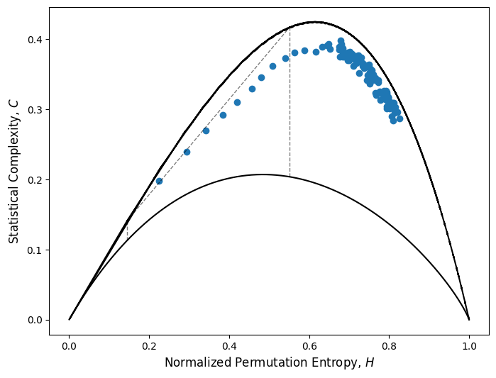
The documentation for HCplots.HCplane lists additional arguments for modifying the styles of the various elements of the plot.

Now supposed we’d like to calculate the \([H, C]\) coordinate for the maximum Statistical Complexity of the x-coordinates of mass 2 of this double pendulum system. One way to do it is to plot the \(H(\ell)\) and \(C(\ell)\) curves to identify what timescale corresponds to maximum complexity, e.g.,

>>> HCplots.HCcurves(H=H, C=C, sampInts=ells)
>>> plt.show()

This gives us the plot:

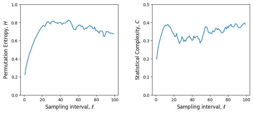
While this is useful when chaotic behavior is expected, to use PECCARY on a timeseries where the behavior is not know, it is better to use the idealized sampling scheme discussed in Section 3.2 of Hyman, Daniel, & Schaffner (2025). These recommendations are to use \(0.3 \lesssim t_{pat}/t_{nat} \lesssim 0.5\) and \(t_{dur}/t_{nat} \geq 1.5\). Since the double pendulum is a chaotic system, we need to approximate its natural timescale by using the utils.tNatApprox function.

>>> tNat = utils.tNatApprox(pend.t, pend.x[1])

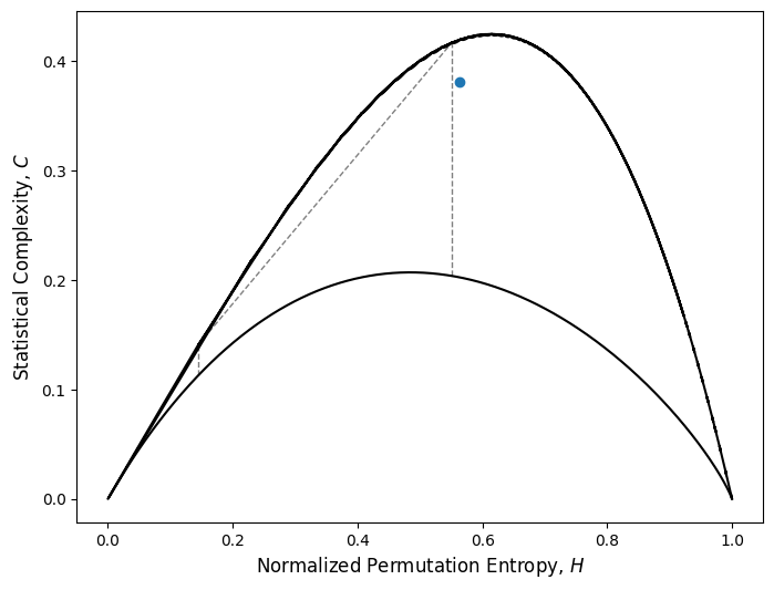
We can convert our desired time resolution ratio of \(t_{pat}/t_{nat} = 0.4\) to a sampling interval using the natural timescale we calculated and the function utils.tpat2ell:

>>> ell = utils.tpat2ell(0.4*tNat, dt=pend.dt)

We can now calculate the ideal \(H\) and \(C\) calues for using:

>>> idealH, idealC = pecc.calcHC(sampInt=ell)
>>> HCplots.HCplane(idealH, idealC)
>>> plt.show()

This gives us the plot of the \(HC\)-plane, which indicates that our timeseries is indeed complex:

In-depth discussion of the choices and interpretations for \(H\) and \(C\) can be found in Hyman, Daniel, & Schaffner (2025). Additional documentation and examples for each function can be found in the User Guide.